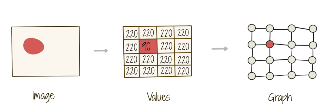
An image is a set of pixel values over a regular grid on a Euclidean plane. A graph (with a chosen adjacent node connectivity) generalizes this, since the pixel values may then lie over an irregular grid (as shown).
Further, a graph may also represent data over a non-Euclidean structure.

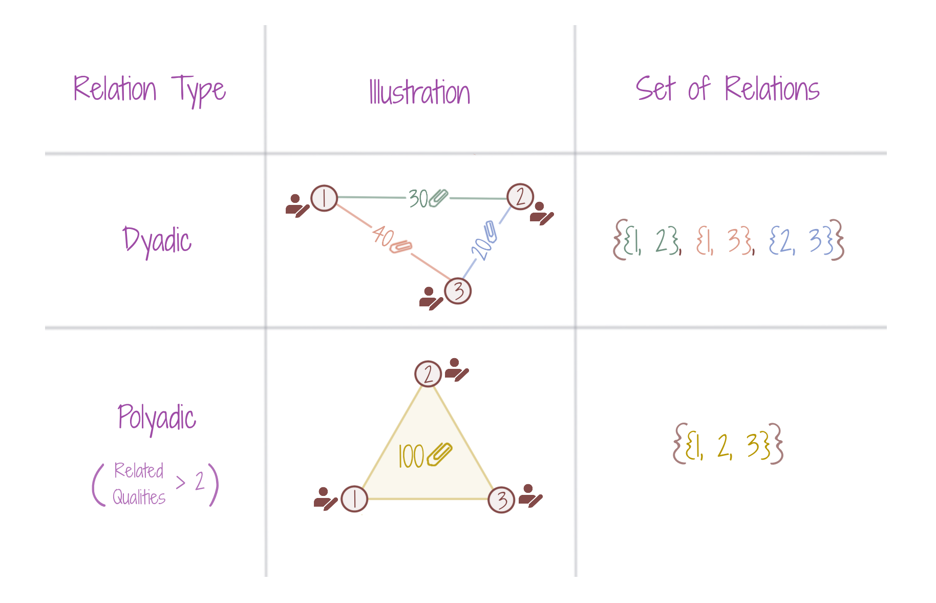
A graph, when connecting 3 entities, explicitly suggests that each pair is related. The edges are thus endowed with pairwise data (features), e.g. citation count of paper authored by 2 researchers. What if three researchers together co-author a paper? We then require a collective feature between the three nodes. This relation is a polyadic relation, modeled by complexes or hypergraphs.
While defining a polyadic relation, both Complexes and Hypergraphs may implicitly suggest the existence of underlying dyadic relations also (through combinatorial construction properties). However, pairwise features do not mandate themselves to be incorporated.

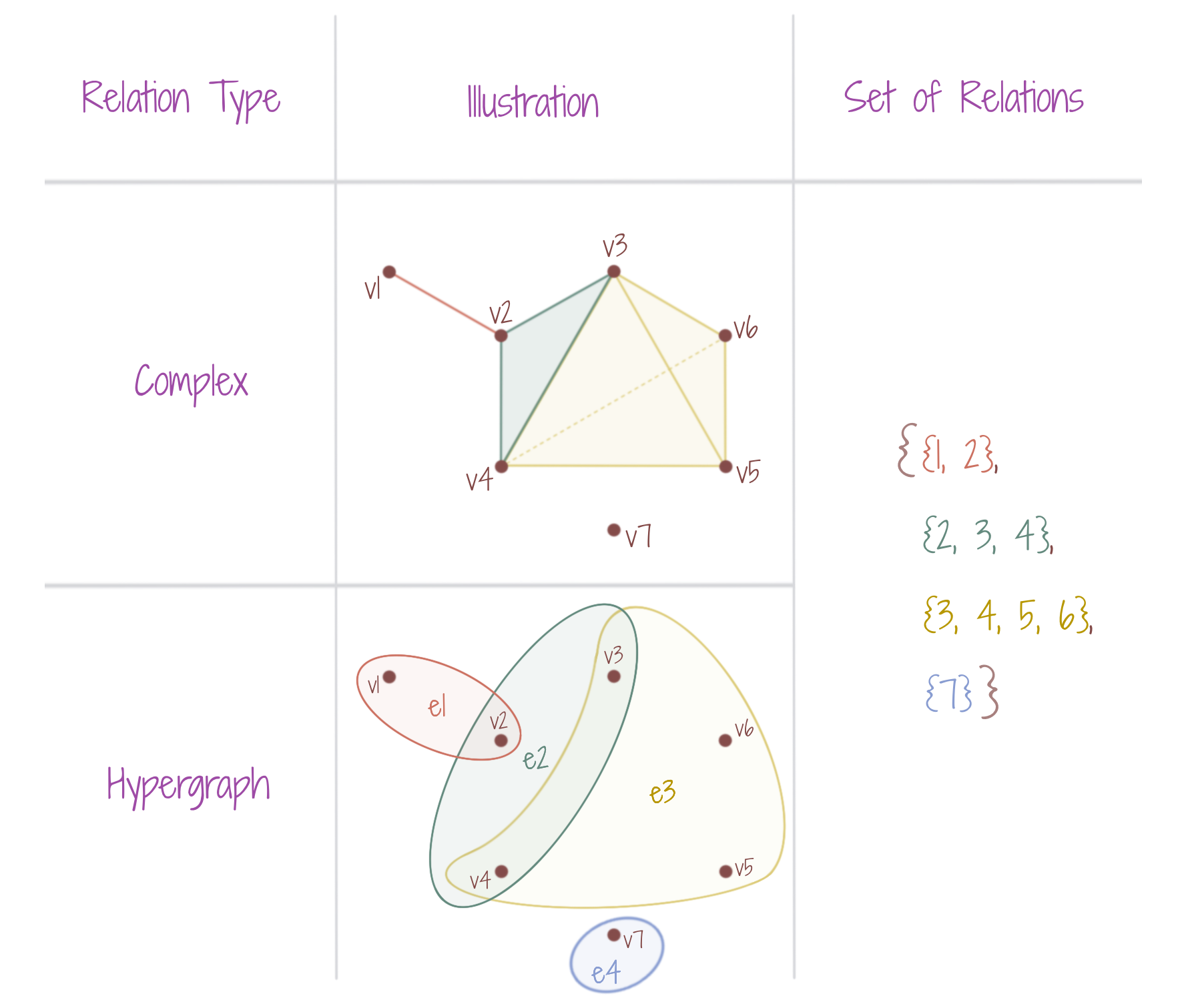
A complex makes use of higher-dimensional structures, like triangles, tetrahedrons (instead of only line segments), while a hypergraph groups multiple vertices (instead of only two), to model polyadic relations. Where a complex would also generally retain the notion of individual line segments as edges, a hypergraph would usually be free from such downward inclusion ideas, and only the sets of connected vertices form hyperedges (e1, e2, e3, e4).
The figure shows an undirected simplicial complex, with an isolated node, and the corresponding hypergraph.

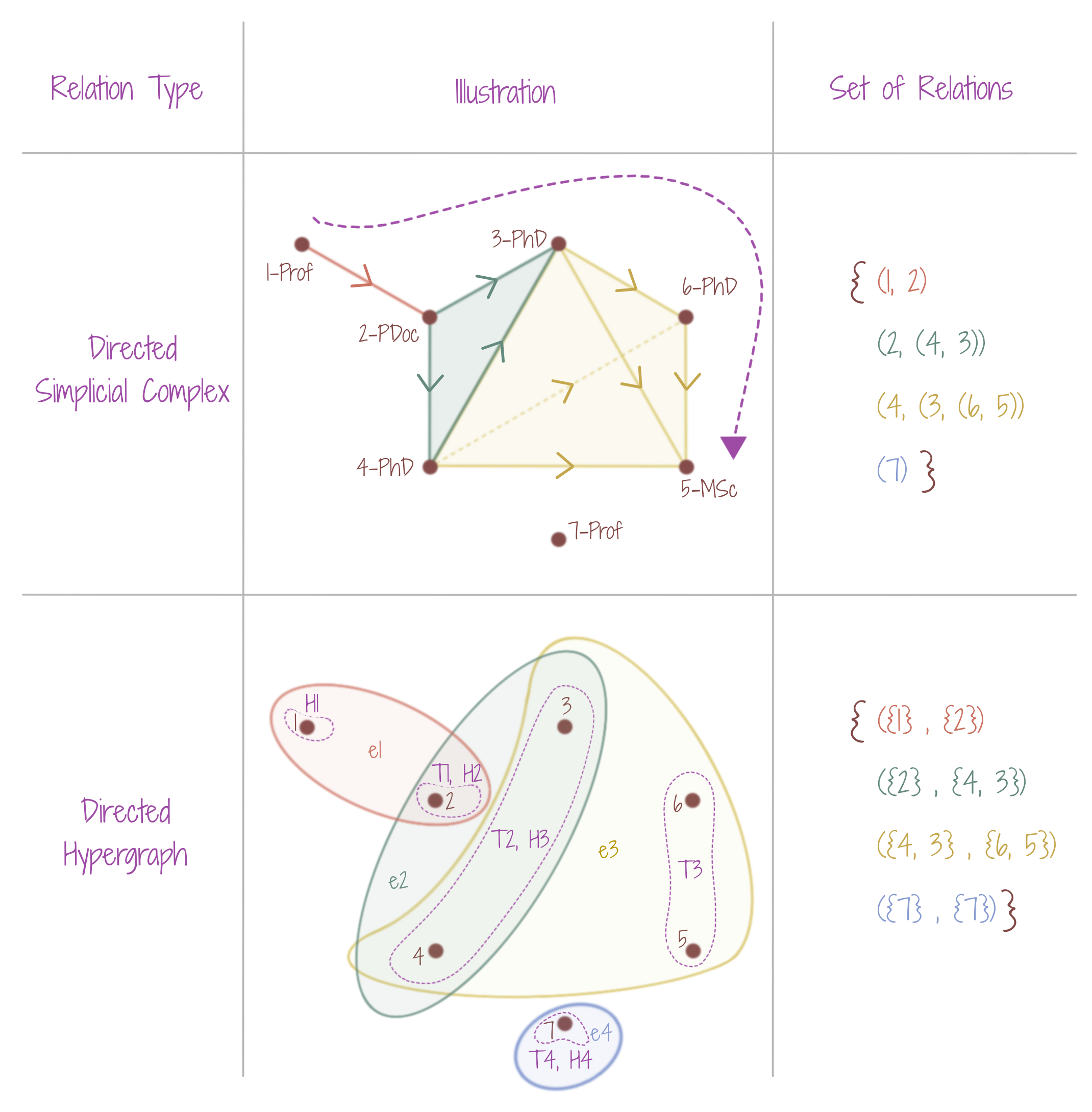
The figure shows an interesting situation, for authoring a research paper through sequential collaboration, using a directed simplicial complex, as well as, a directed hypergraph. A professor (node 1) gives the first paper draft to his PostDoc (node 2), who then collaborates with his PhD students (nodes 3 and 4) to make further edits. The paper then passes to another PhD student (node 6) and a Masters student (node 5), who collaborate further, to put together the final version of the paper. Due to the directionality over the complex/hypergraph, the paper does not travel back to the main Professor (node 1), and the other Professor (node 7) never collaborates.
Note that if the direction between node 2 & node 3, had been reversed, this would mean that the paper never passes onto the PhD student (node 6) and the Masters student (node 5) for collaboration, once it has been initiated by Professor (node 1). The PhD students (nodes 4, 5, 6) and the Masters student (node 5) although can collaborate for writing a research paper, but independent of Professor (node 1) and PostDoc (node 2).

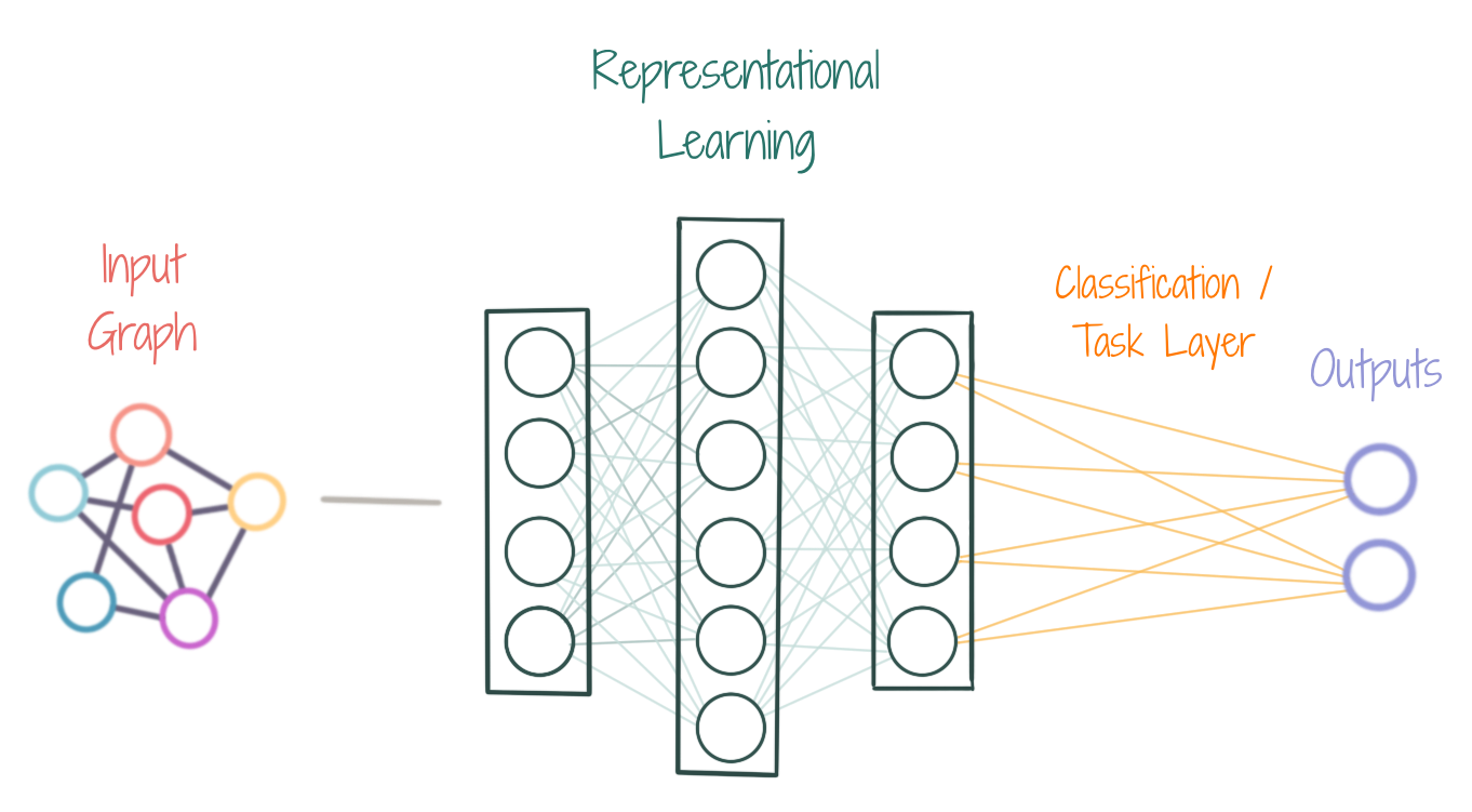
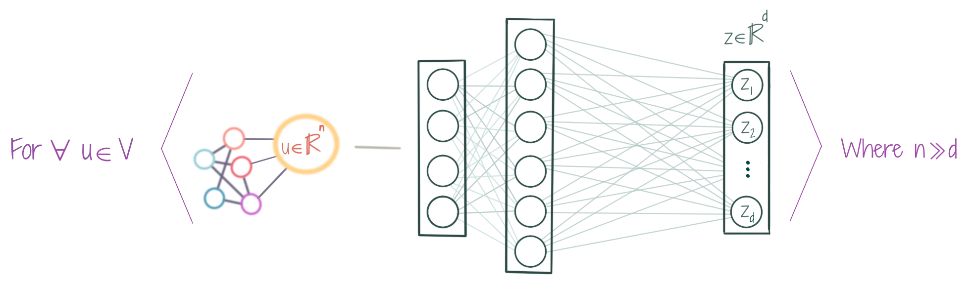
Mostly, a GNN learns a multidimensional (Rd) embedding/representation for each node of the graph, which is then used to perform a certain task, e.g. classification.

Representational Learning is the automatic learning of Features/embeddings (with an NN) instead of engineering them manually. In case of a GNN, the embedding of the node u is learnt by taking into account the local graph structure around u, i.e. the information contained in the neighboring nodes and edges of u is also encoded in z.

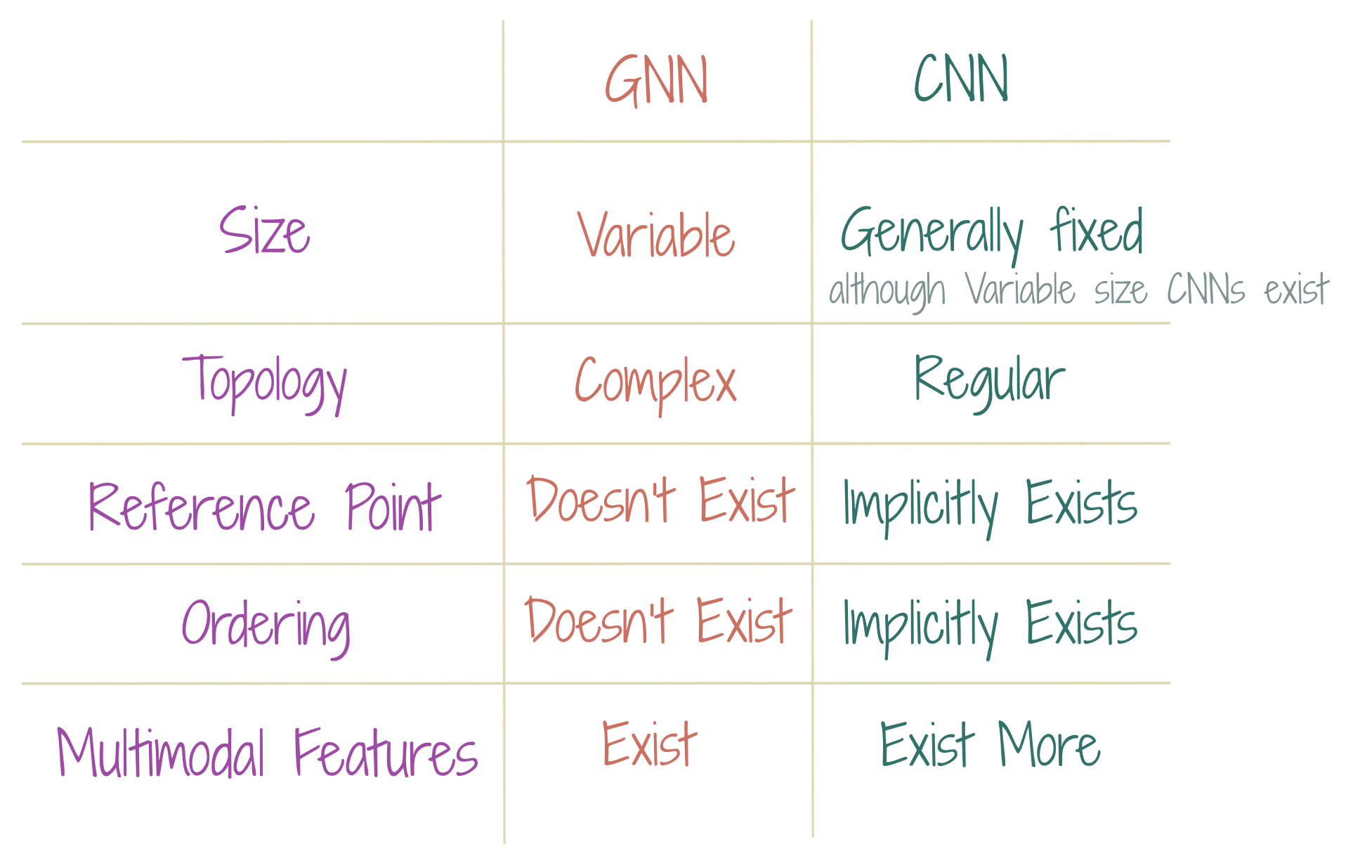
The table shows key differences in the characteristics of the inputs, admitted by GNNs and CNNs. It is clear that the GNNs allow a wider variety in their input data.
The multimodality, should, roughly be understood as, being of different types. However, the way the term has been used with CNNs versus that with GNNs, invites some mention. Usually, with CNNs and in the field of CV/ML, multimodality has referred to the types that arise from distinct modes of human - computer interaction, e.g. textual, visual, auditory. However, in GNNs, multimodality may simply mean different types of data, where these types may even come from the same mode of human-computer interaction, e.g. in a knowledge graph. This essence of multimodality can be seen implicitly within the CNNs, e.g. different parts of a face (nose, eyes, mouth, head, cheeks) can be seen as multi-modal features, as they produce modes in the joint probability distribution of the facial images. In principle, this is very justifiable; however, in practice, the term has precluded CNNs for such purposes.

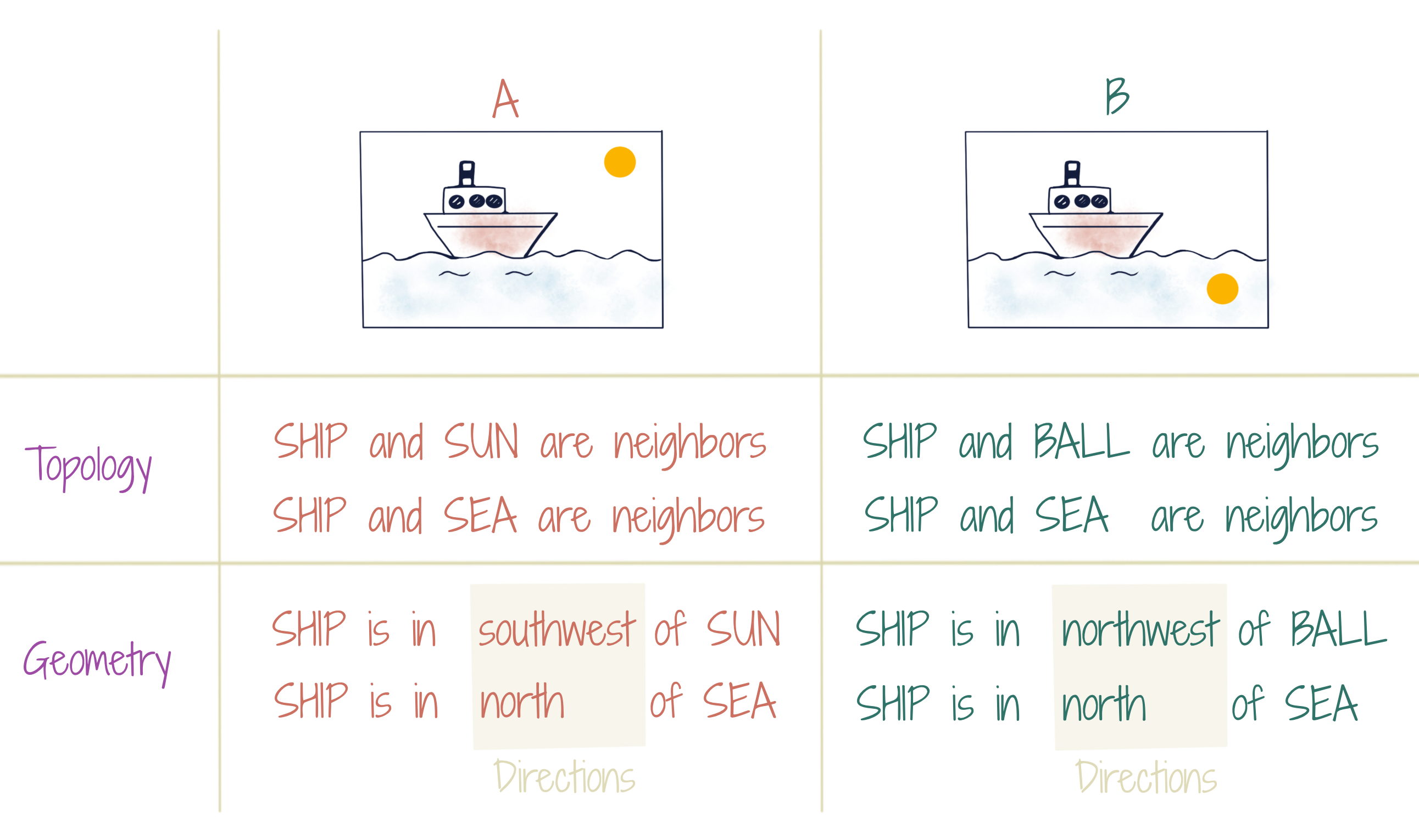
Using only topological information (conventional GNNs), the ball in image-B can be predicted as the sun. Adding explicit geometry (like in transformers) resolves this, while implicit geometry (like in CNNs) may or may not.

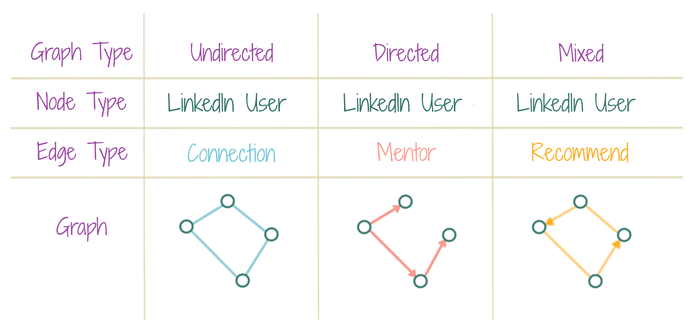
The edges in a graph can be directed, undirected, or both (mixed). An undirected edge conveys a two-way relationship, while a directed edge indicates only a one-way connection.

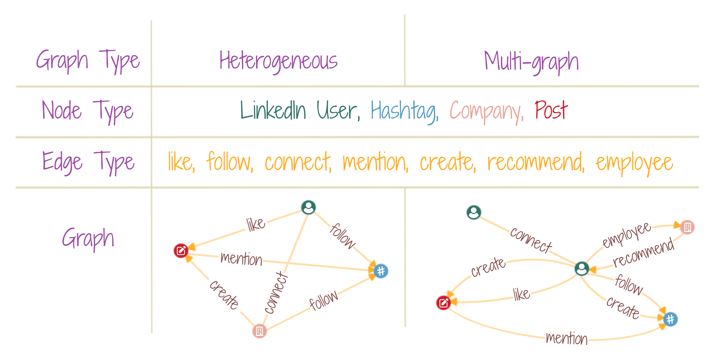
By default, all nodes (and edges) in a graph are of the same type(s), and only one edge is allowed between any two nodes of a graph, be it directed or undirected. A heterogenous graph allows nodes to be of different types, and so, for the edges. A multi-graph allows for multiple edges between any two nodes in a graph. The figure shows examples from a conceptual LinkedIn network. Each example has multiple node types (individual user, company, post, hashtag) and multiple edge types (like, follow, connect, mention, create, recommend, employee). Some edge types like connect are undirected, since they indicate a two-way relationship, while those like follow are directed, since it’s not always necessary that two connected entities follow each other. A user can both create and like a post; thus, two edge types are possible between users and posts. However, these edges are of a directed variation, since only a user may create/like a post, and not vice-versa.

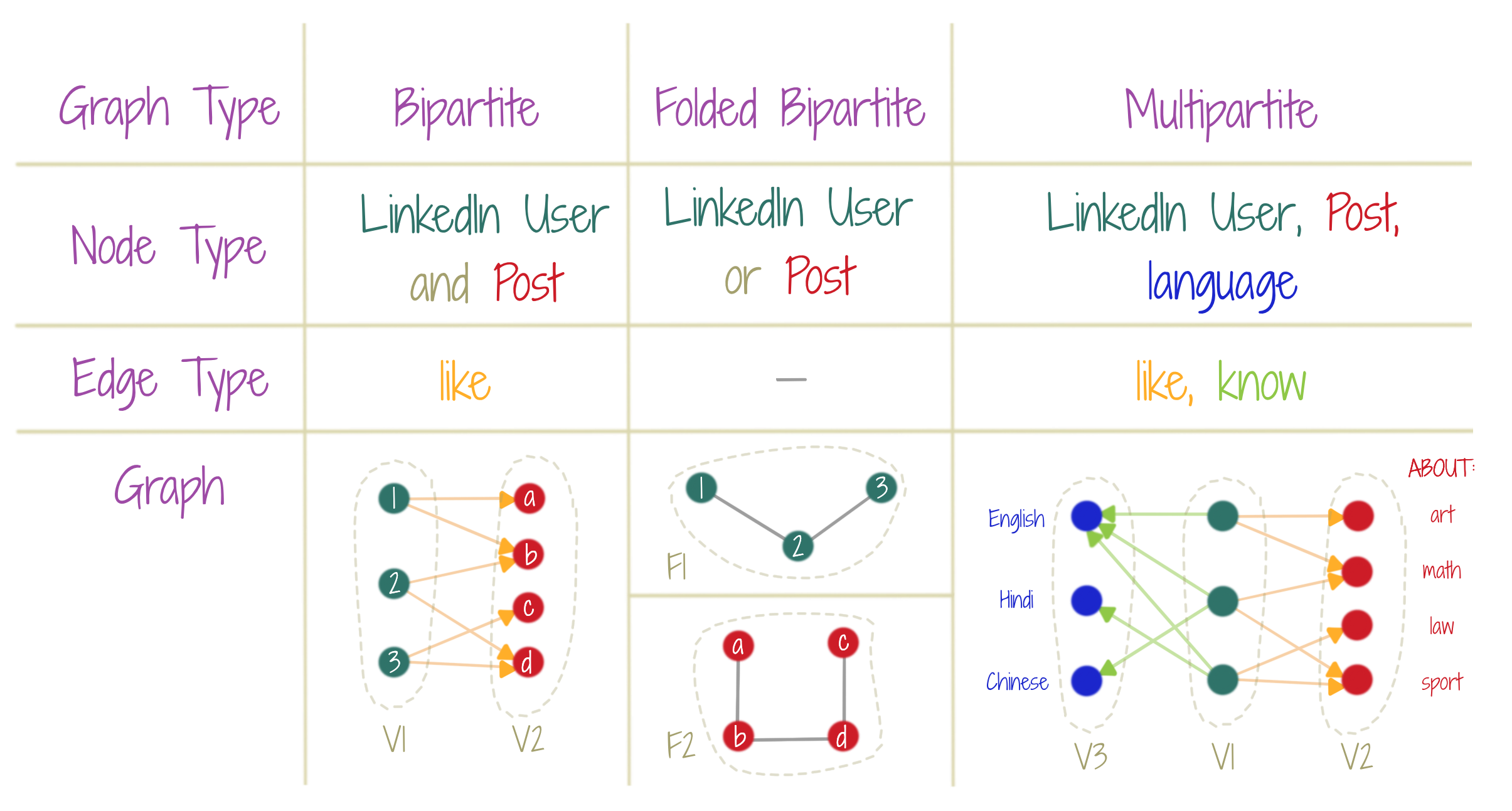
A bipartite graph has two disjoint sets of nodes, such that no nodes within each set are connected. A multi-partite graph extends this idea to more than two disjoint sets of nodes. A folded bipartite graph establishes a sense of (indirect) connections between the nodes of each disjoint set of a bipartite graph. Thus, in the figure, the folded bipartite graph for the red nodes, shows that red nodes (a,c) are not (indirectly) connected through green nodes, while (a,b), (b,d), (c,d) are (indirectly) connected. A similar folding operation may also be applied to the disjoint sets of a multi-partite graph.

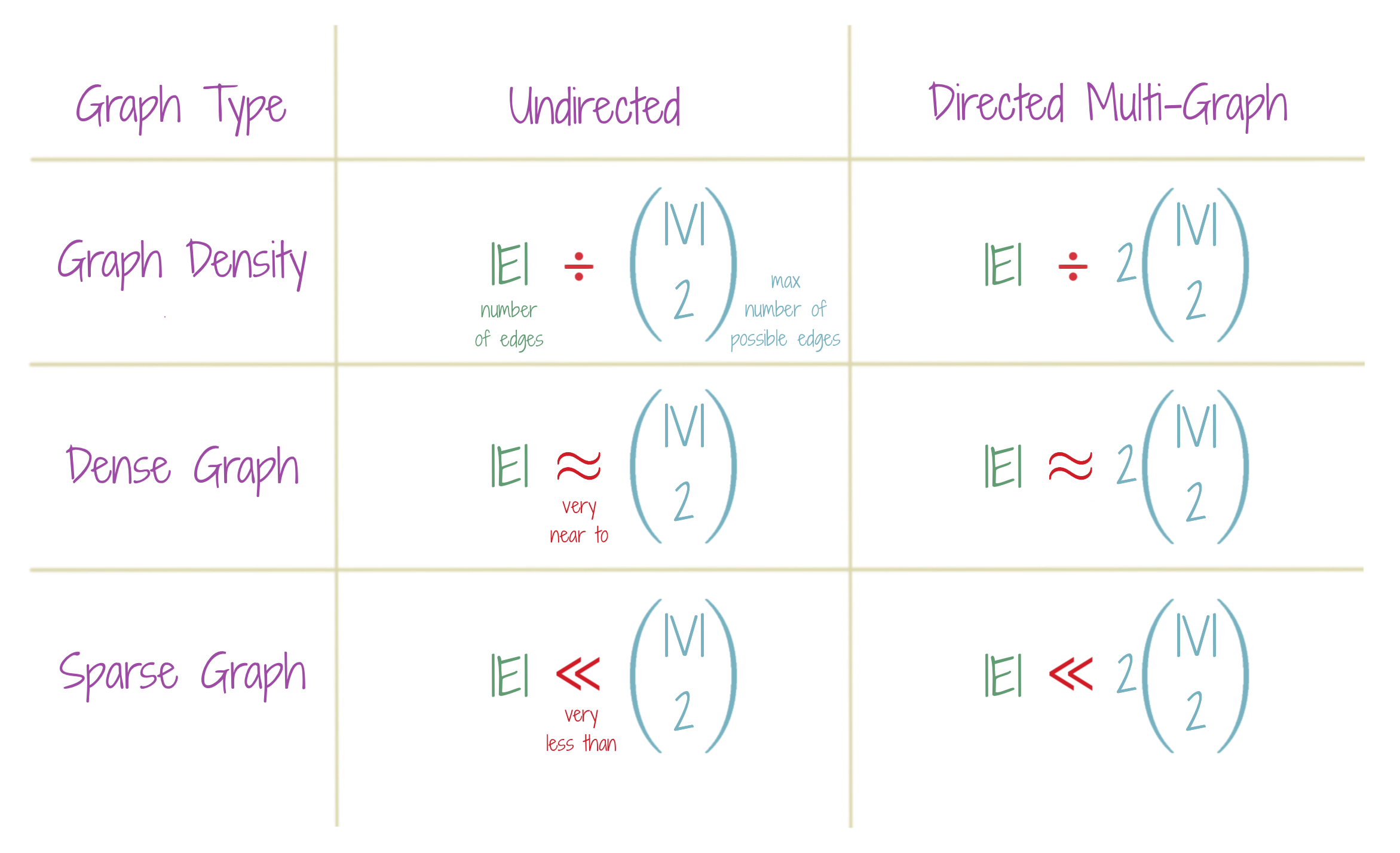
Density of a graph is a measure of how connected a given graph is, in comparison to what it possibly be. A sparse graph is very less connected, while a dense graph is almost maximally connected. Note that in the case of directed graphs, the maximal number of edges are twice than those in undirected graphs, in order to account for directedness. All given expressions are for simple graphs, i.e. multiple edges are not allowed between any two nodes.

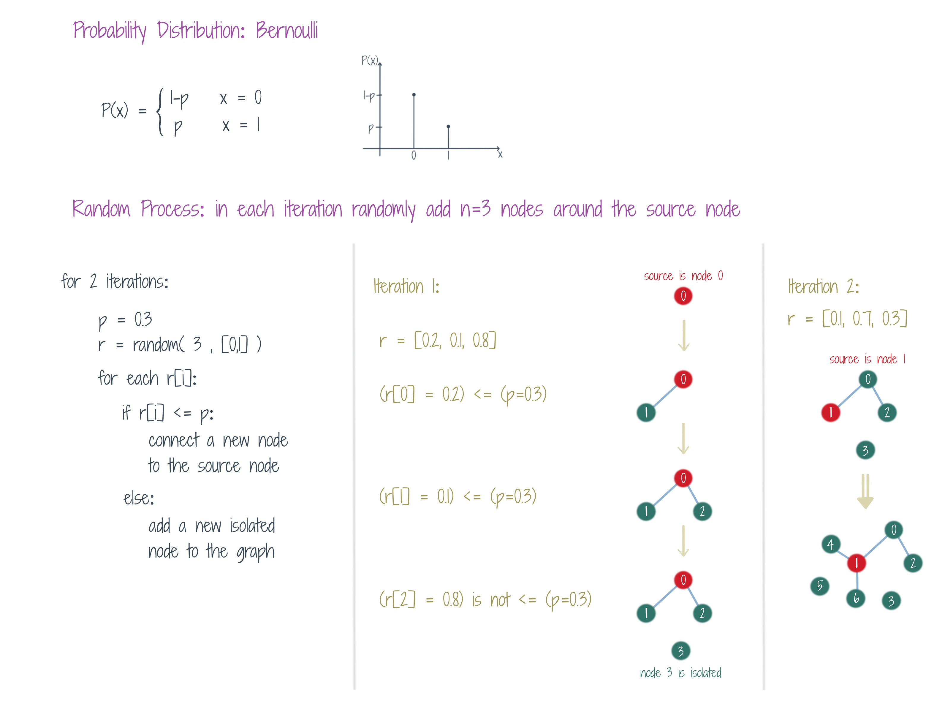
The figure shows how the edges of a simple graph may be generated (independently of other edges) through a random process, where at each processing time-step (iteration), the random variable follows a Bernoulli Distribution. The figure shows 2 such iterations. Criteria may also be defined to add/delete nodes of the graph, through another random process. The Erdos - Renyi Model is a famous random graph generation model, which is used to provide guarantees on the existence of properties of interest, for a general family of graphs.

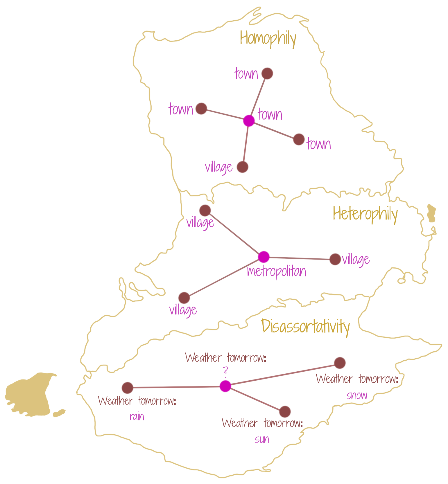
A homophilic graph contains similar neighbors (nodes) to a given node, while a heterophilic graph is likely to contain dissimilar neighbors to a node. In both cases, however, a node receives useful/important information from its neighbors. When the neighbors of a node are such that they do not provide any useful information, the graph is disassortative. Disassortative graphs, therefore, often require access to long-range relations for gaining useful information. The figure shows the homophilic and heterophilic concepts through nodes that may depict towns, villages, metropolitan cities in a country. The disassortativity is shown through a hypothetical construction, where saying everything about the weather forecast, does not give any clear idea for weather prediction, and therefore, is not useful.
Note that homophilic graphs are also called associative graphs, since a node of a given type is likely to be associated with the nodes of the same type. Under similar parlance, heterophilic graphs are also called dissociative graphs, since a node of a given type is likely to be not-associated to nodes of the same type.

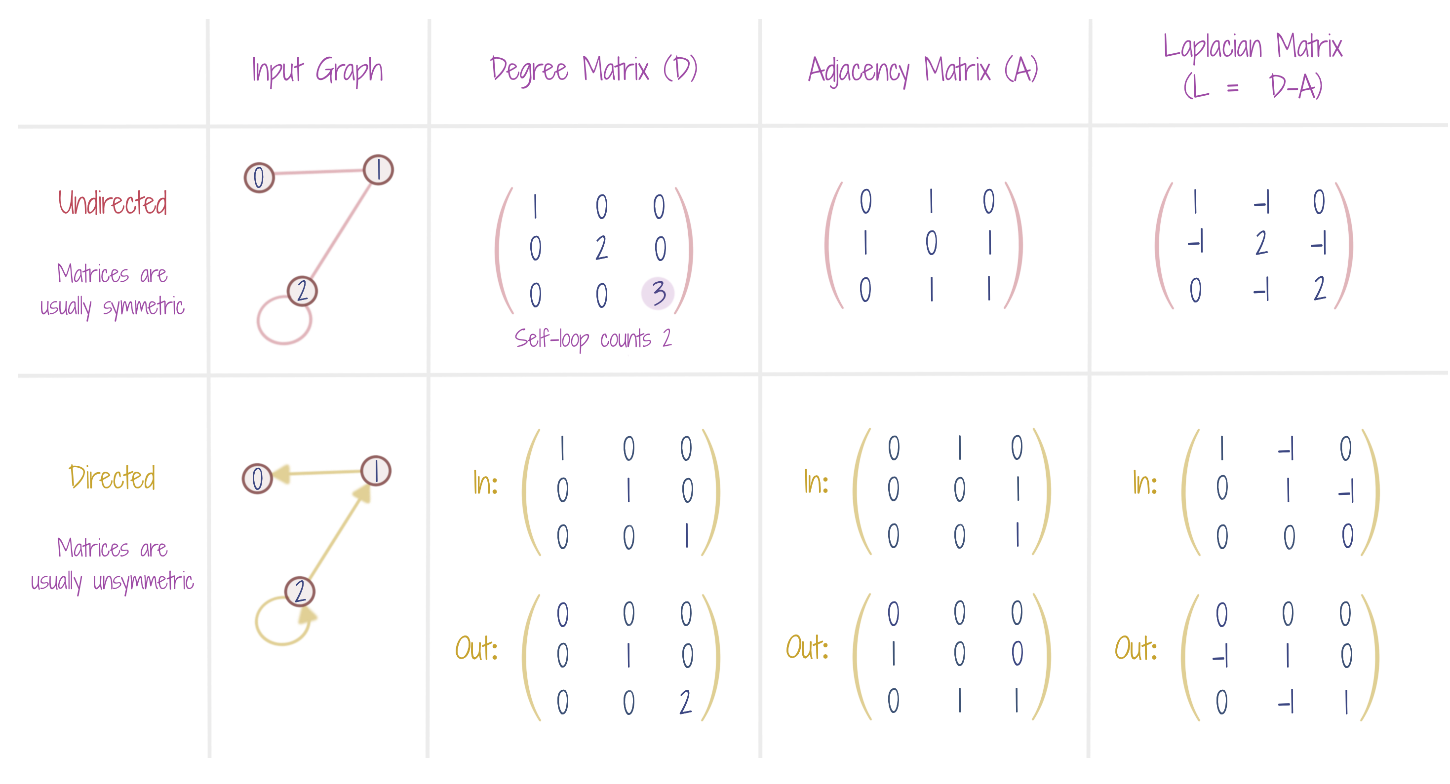
A degree matrix tells the number of neighbors for each node, while an adjacency matrix tells which nodes are the neighbors. The Laplacian matrix, say, being applied to a function f, tells how much on an average the value of f at a given node i is greater than the value of f at i’s neighbors.
The Laplacian Operator can also be given an interpretation as being the divergence of gradient of the function f (scalar field). This is by the definition of the Laplacian in terms of the gradient operator 𝝯. If one imagines f as a flow function, a near-zero Laplacian (on a region) would then mean that the flow does not form a sink or source (in that region), or, in other words, the flowing fluid does not contract or expand (in that region).

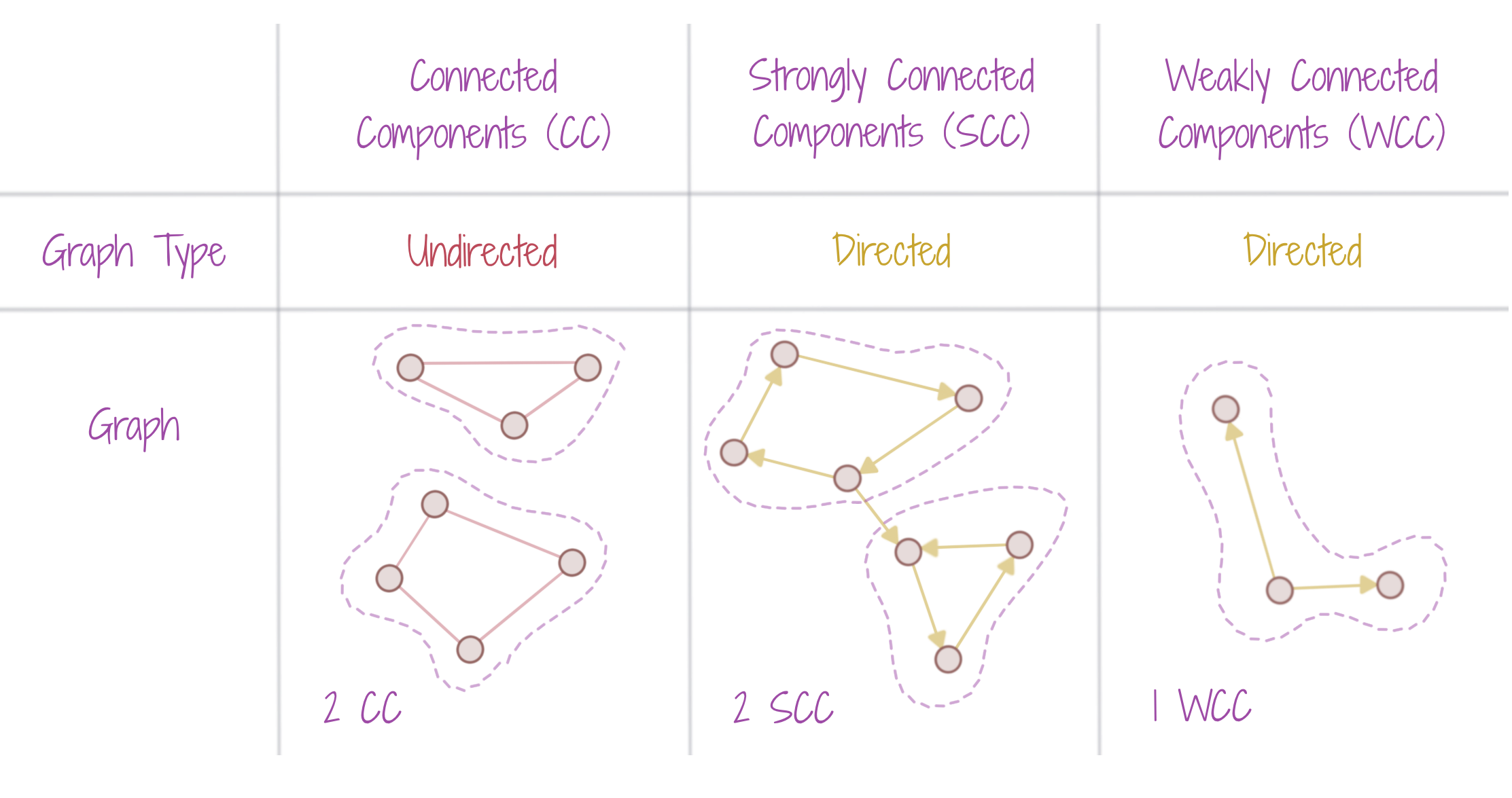
A connected component in an undirected graph is a subgraph in which there is a path between every pair of nodes. To extend the notion to directed graphs, we have strongly and weakly connected components.
Note that the basic idea of a connected component is that we can traverse from any node to any other node in the component. It’s just that we have more specific terminology for directed graphs.

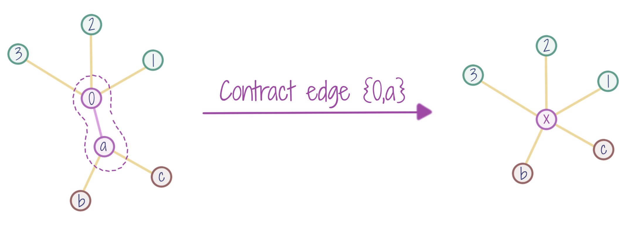
An edge in a graph can be contracted by merging the two connecting nodes to a single node. The figure shows that the edge connecting the nodes 0 and a, is contracted, and the new merged node is x. The neighbors of new node x, are a union of the neighbors of nodes 0 and a.

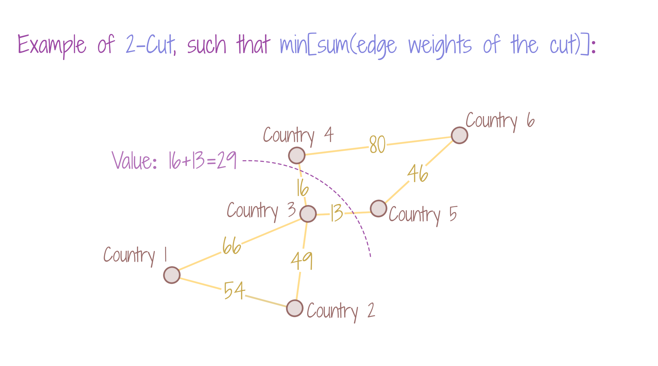
The figure shows an example of min 2-cut, the graph is thus partitioned into 2 connected components. The graph nodes represent countries and edges represent the value of trade occurring between the countries. We wish to form two country coalitions, such that discontinuation in trade partnerships after the coalition, has minimal effect on the trade, i.e. the partitioning of the graph is minimal in edge values.

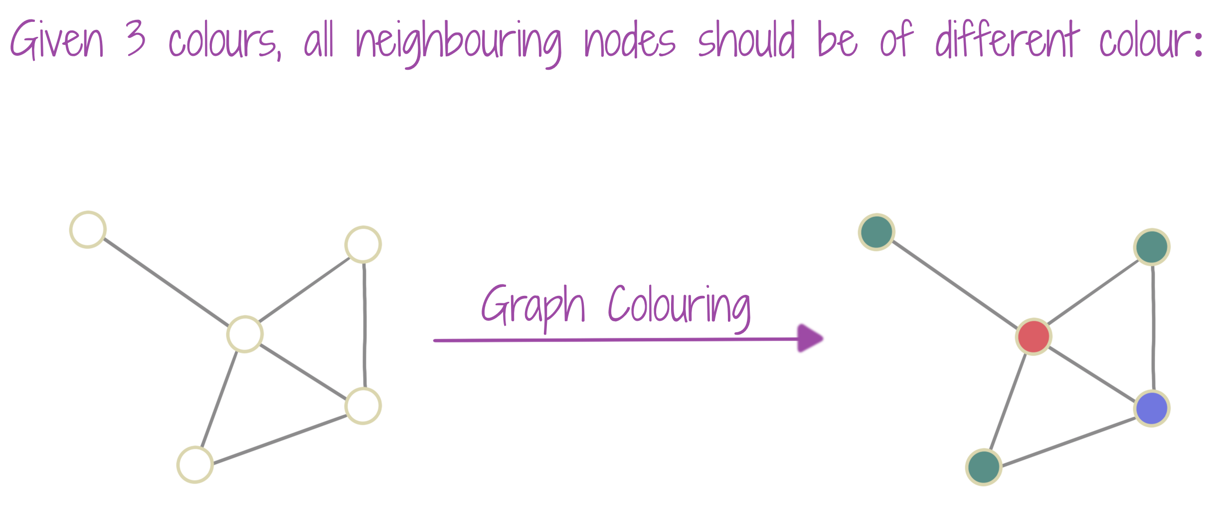
Graph coloring is the process of labeling nodes of the graph into node types (called colors), according to the constraint that no two neighboring nodes are of similar type (color). It is one of Richard Karp’s 21 NP-complete problems. In a more general scenario, one can also label edges with a given set of types (colors), according to a new constraint.
Graph Coloring algorithms are used in Computer Science to solve problems, where we have a limited amount of resources, with some restrictions on how they can be used, e.g. network scheduling, register allocation. Sudoku puzzles can also be seen as a graph coloring problem, since the resources (numbers) are limited, and they have to be used as per the constraints of the sum along rows, columns, and 3x3 squares. Training a GNN which can provide good approximation guarantees to graph coloring problems, can be challenging.

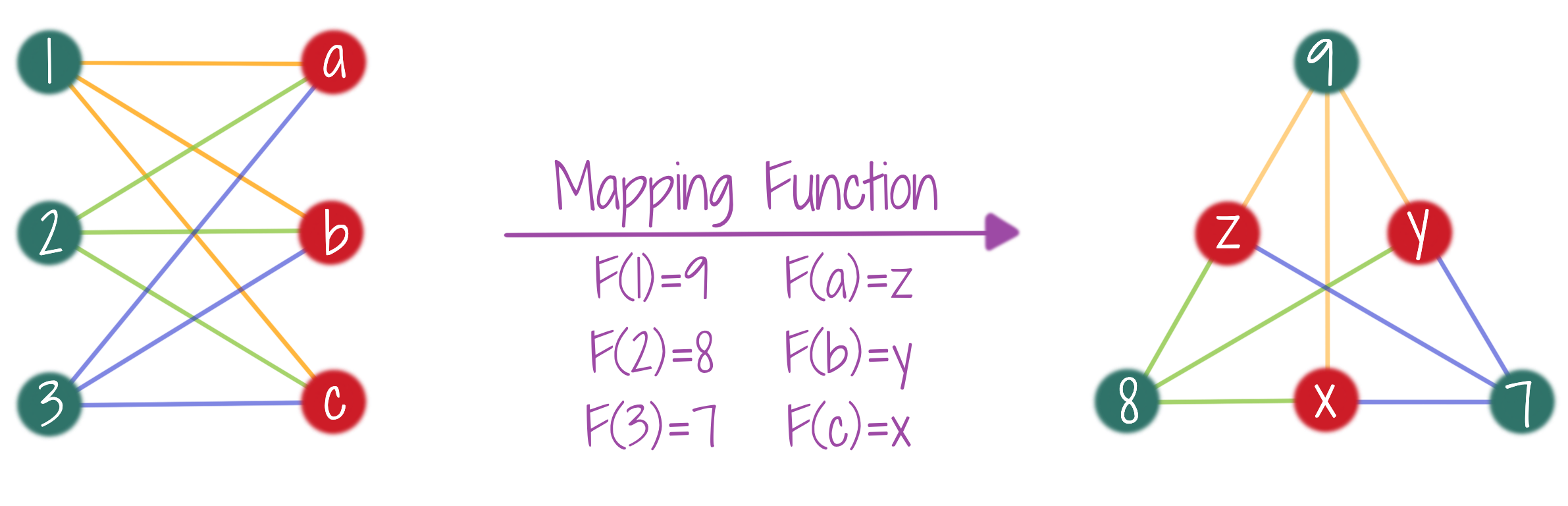
Two graphs are isomorphic, if they are essentially the same graphs (topologically), but with different node names. The figure shows two isomorphic graphs and a mapping function that matches the nodes across these graphs. Note that the topology (connection pattern) in the two graphs is the same. Graph Isomorphism has emerged as a very useful concept to study the expressive power of GNNs, i.e. which properties of graphs GNNs can’t recognize.

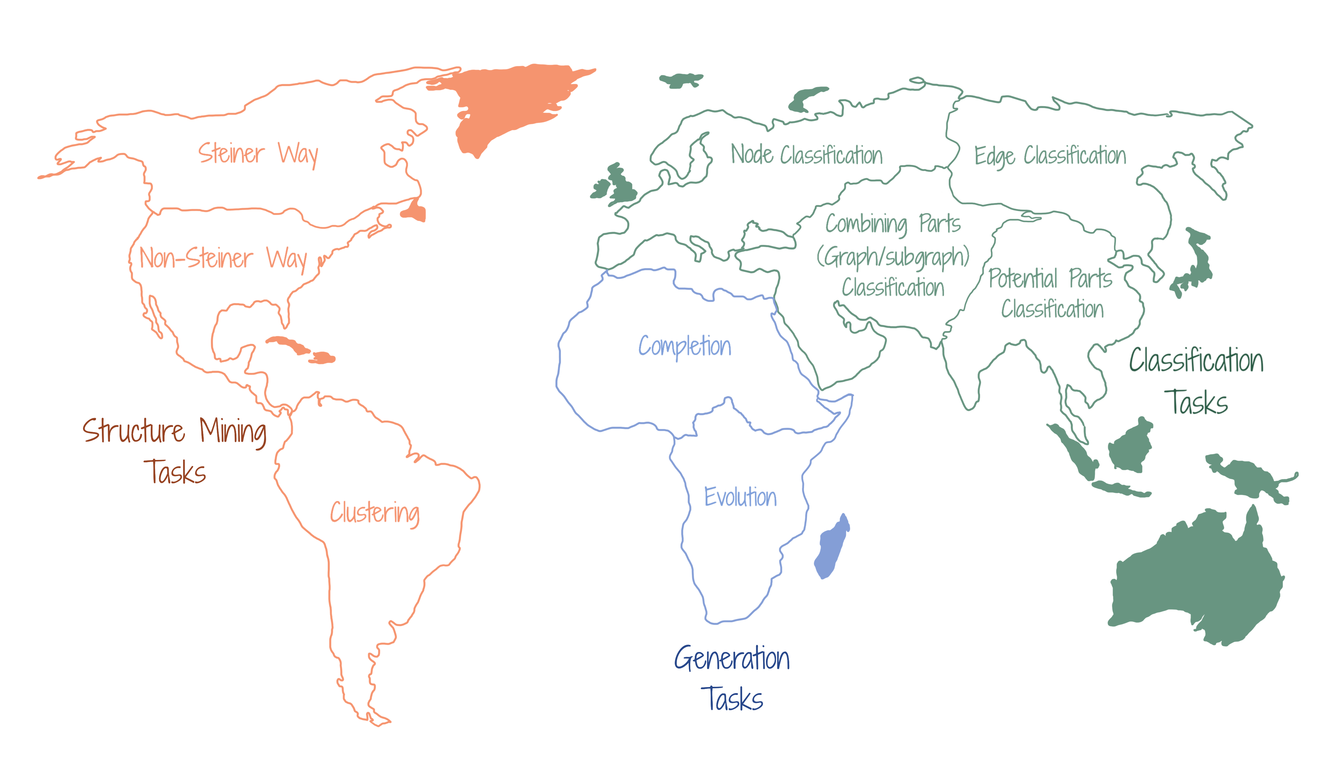
Graph neural networks (GNNs) can be used to learn multiple types of tasks for graph-input data. These learning tasks can mostly be of three types - (a) Classification (b) Structure Mining (c) Generation. In classification tasks, the aim is to assign some part (or whole) of the graph to known classes. In structure mining tasks, the aim is to find the part (or mild augmentation) of the graph that may most appropriately represent a target concept. In generation tasks, the aim is to generate new graphs.
A graph may be generated with a completing or a completely new topology and new node and edge attributes, or just with new node and edge attributes, while keeping the same topology. With a new topological structure, a graph can be generated unconditionally, or conditionally (from an existing subgraph) to reflect a chosen concept. Alternatively, a graph may be evolved from an existing graph, keeping the same topology, but modifying the node and edge attributes, to model some system dynamics.

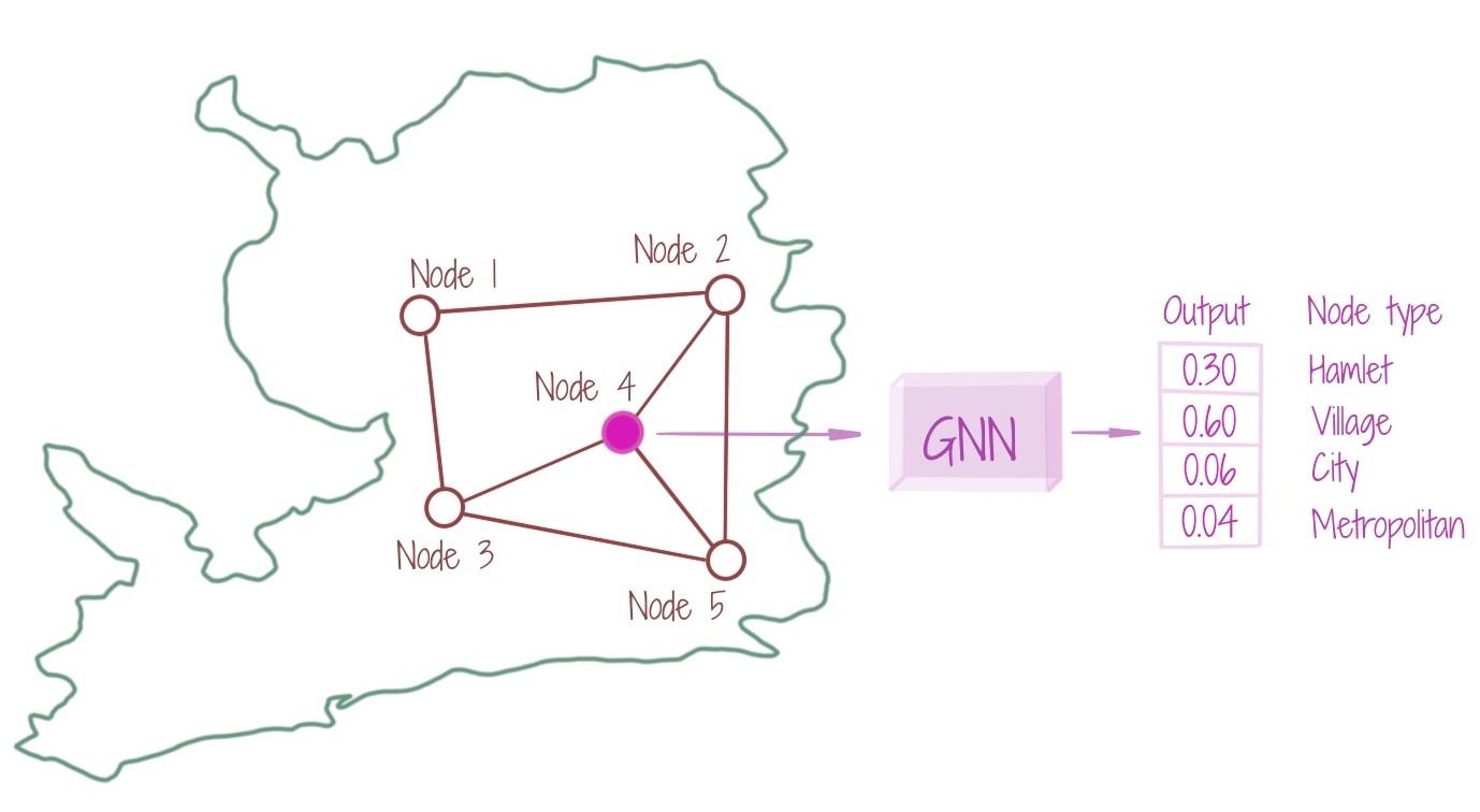
For an input graph G, a GNN is learnt to assign a class (from a pre-chosen set of node classes) to each given node n. The assignment is made considering the topology of the node n, i.e. its neighboring nodes. The neighboring nodes, in turn, come with their own topology. Thus, a node n, indirectly encompasses the entire graph topology. The figure shows that the pre-chosen set of node classes is {hamlet, village, city, metropolitan}, and the node is assigned the class village based on the highest probability output from the GNN. Node feature learning (used in node classification) is widely used in most other GNN learning tasks as well.

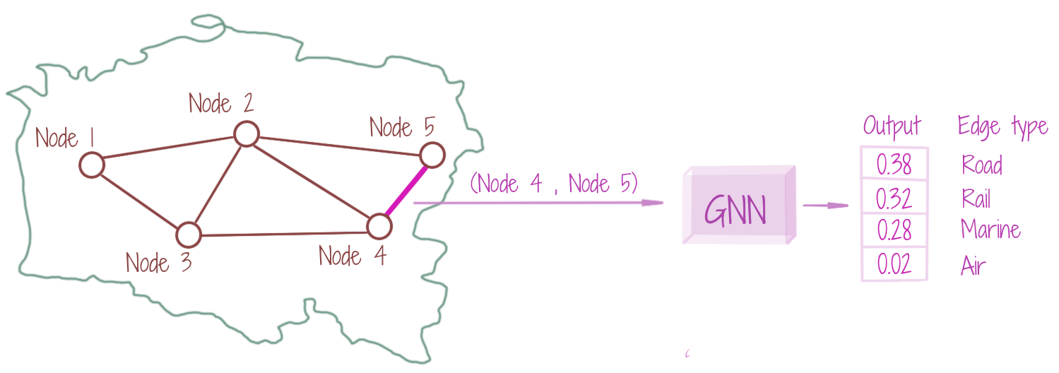
For an input graph G, a GNN can be learnt to assign a class (from a pre-chosen set of edge classes) to each given edge e. The assignment is made considering the topologies of the connecting nodes, which indirectly encompass the entire graph topology. The edge classification is thus dependent on the node-level representations. The figure shows that the pre-chosen set of edge classes is {road, rail, marine, air}, and the edge (between nodes 4 and 5) is assigned the class road based on the highest probability output.

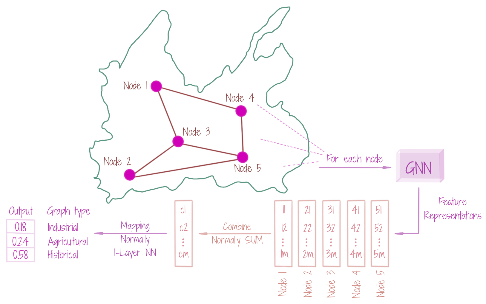
We may assign a class to an entire graph, or a subgraph (which is not simply a node or an edge). The procedure typically starts with the learning of node-level embeddings, and then combining them with a function of choice, to build the representation for the graph (subgraph). These combined embeddings can be converted to class-specific probabilities by a simple neural network. In the figure, the nodes come from {village, metropolitan, hamlet, city}, and based on the corresponding feature representations, a selected area may belong to {industrial, agricultural, historical}. The node representations take into account the connecting edge types that come from {road, rail, marine, air}.

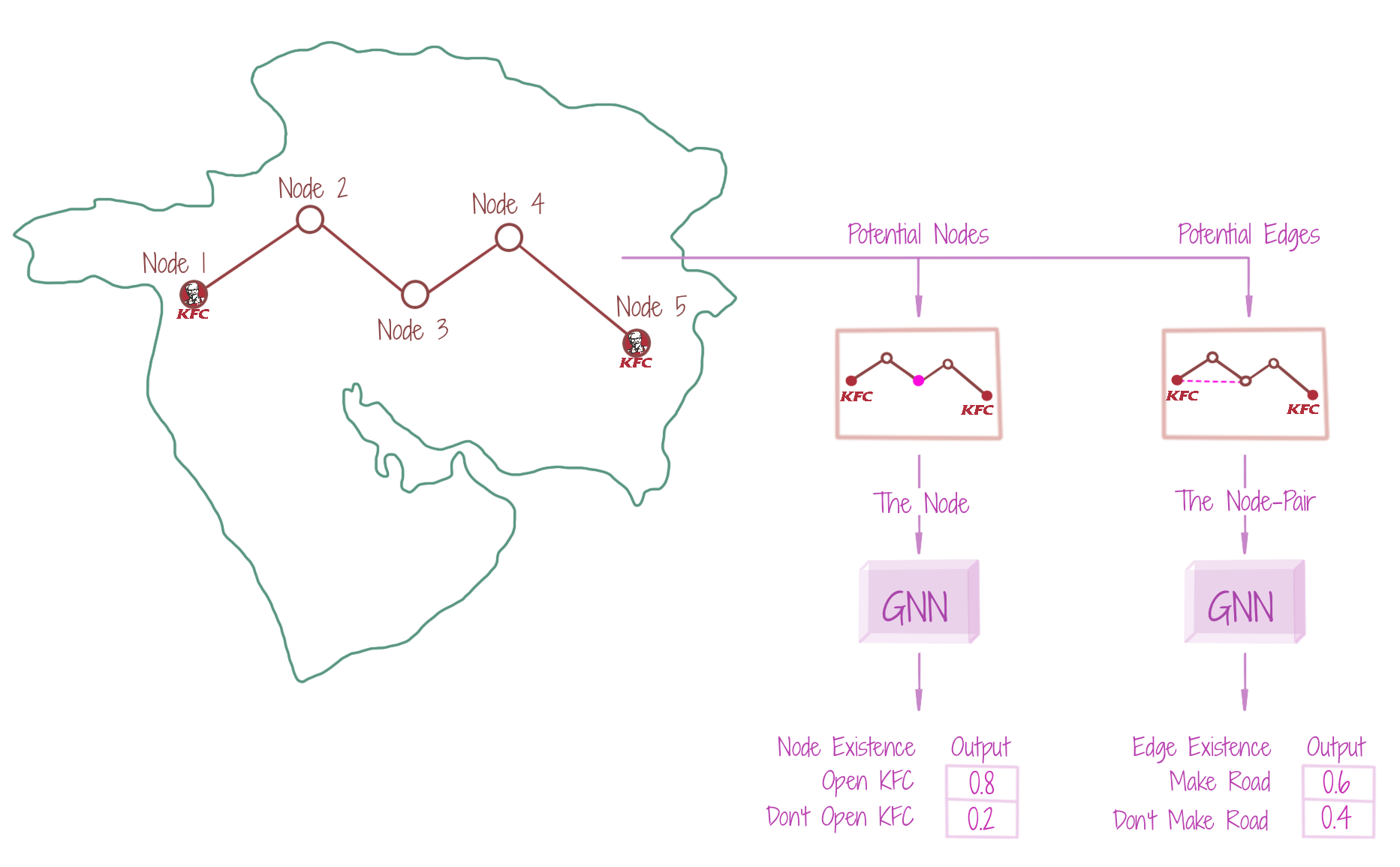
For an input graph G, we may want to predict if a missing edge should exist or not, and if a given node may have a type T. The former can be seen as a (binary) edge classification problem, while the latter is essentially a (binary) node classification problem. Such binary classification problems have an essence of finding the existence or the nature of potential parts of the graph, when the parts are topologically known. The figure attempts to depict the scenario, where we wish to decide if a given property (node) should be designated for KFC (node type), and whether a road (edge) may be established between two given eating outlets. The (binary) edge classification is often referred to as the link prediction problem, useful in recommender systems. For instance, an edge may be established between a user and a movie, if the user likes the movie, else not.

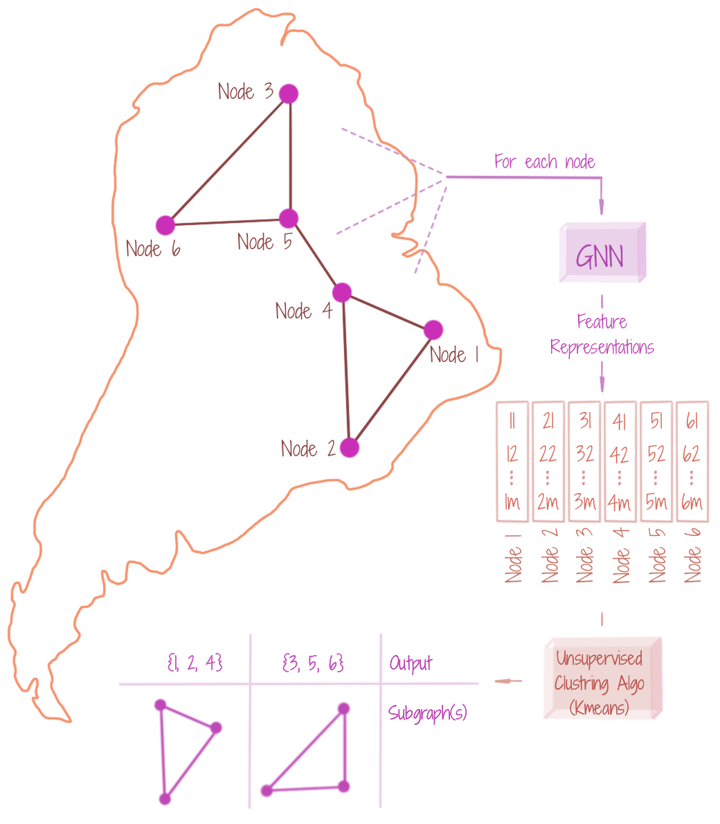
Given a graph G, we may want to find subgraphs reflecting similar concepts. We can achieve this by clustering over the node-level feature representations (learnt through GNN), using unsupervised algorithms like K-means (or spectral clustering if the features seem to be in a non-compact geometry). The node representations take into account the connecting edge types also. Note that the GNN learning objective here, has no notion of similarity of subgraph-level representations. However, such a criterion may be incorporated using metric learning over the clusters.

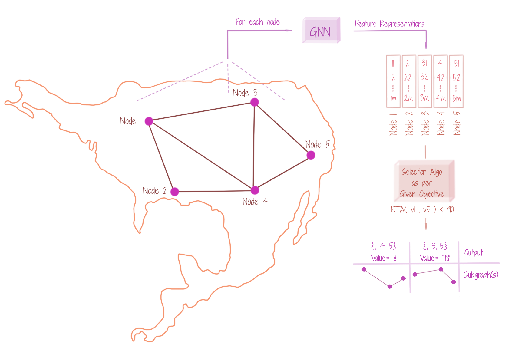
For an input graph G, we may want to find a subgraph matching a specific objective, which may not be directly derived from the node and edge attributes. For instance, the figure shows that we want to find the subgraph connecting towns v1 and v5, such that the ETA (estimated time of travel) is less than 90 minutes. Here, an edge e between any two nodes n and m, carries the attribute of amount of traffic / roundabouts / railway barriers. Thus, it would be advisable to learn this in a data-driven manner, using GNNs. We would again collect the node-level representations (which indirectly consider the network topology with connection types), and design an appropriate subgraph selection algorithm that would translate any selected subgraph to a time estimate. There might be multiple outputs, each satisfying the given criteria. Note here that we do not consider any graph expansion for finding the optimal subgraph, and hence, subgraph mining in non-Steiner.

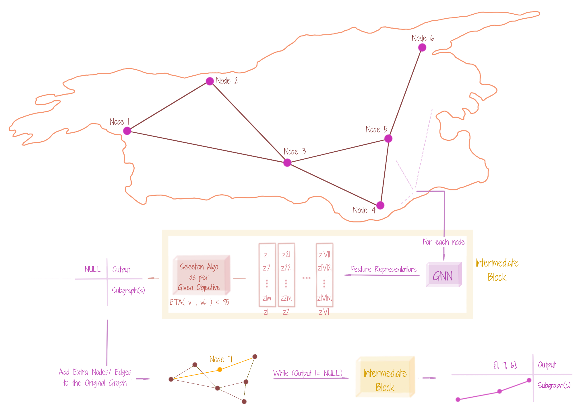
For an input graph G, when we want to find a subgraph matching a specific objective, using data-driven procedures, we may land into a situation where no subgraph matches the criteria. In such cases, it may be interesting to somewhat expand the graph (to additional nodes and edges), in a manner that including these new nodes and edges, might increase the possibility of finding the optimal subgraph. Since we consider additional graph entities for optimizing our objective, the mining is Steiner. The additional entities may be called Steiner nodes and Steiner edges. The figure shows that for optimizing through a potential superset of nodes and edges, one would need to iterate on the typical non-Steiner structure mining procedure.
We emphasize the Steiner-way structure mining, due to recent success in AI methods for proving mathematical theorems, where estimating an expansion of the concept is very helpful. Alternatively, it can be seen as an expansive reasoning mechanism, which tells us that if something is not happening, what more might make it happen. The Steiner-way structure mining has a generative sense, since extra nodes and edges are augmented to the graph. However, the generation may be somewhat limited.

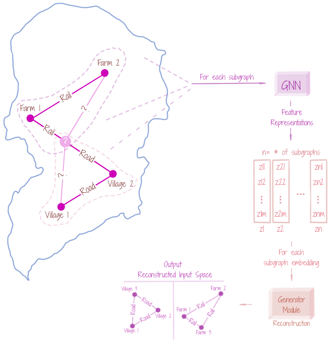
Given a dataset of graphs, a distribution can be learnt over those graphs, and a new graph may be unconditionally generated, by sampling from that distribution. A new graph may also be conditionally generated (from the same distribution), for instance, to complete a partial graph. The graph generation may be done sequentially (usually achieved through Reinforcement Learning / RNN-based procedures), as well as, in one-shot (mostly through encoder-decoder style frameworks). The figure shows that a GNN can be used to learn embeddings (encodings) of the various (randomly-selected) subgraphs (of the input graphs), which may be then passed to a Generator (Decoder) module, learning to reconstruct the graph unconditionally or conditionally. GNN-based graph generation has analogues to data-driven image and 3D mesh model generation, where the first aim is to learn a well-structured distribution of the input space, to sample from, later. Note that graph generation (for completion of a graph or a completely new graph) invites a new topological structure.

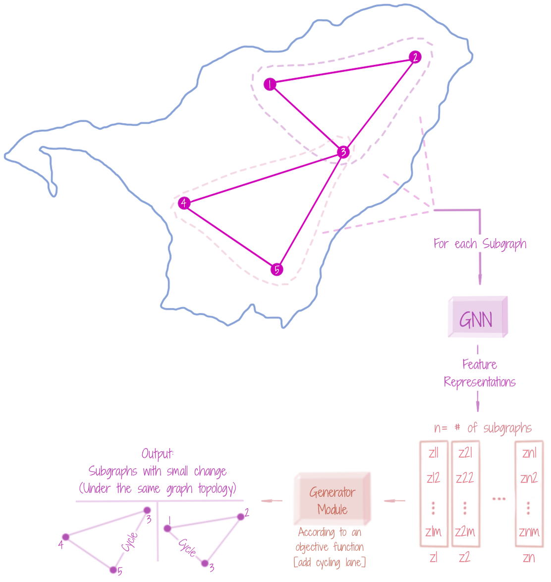
A graph may be generated not to add or construct a new topological structure, but only to update its node and edge attributes, under the same topology. This is called graph evolution, and is generally used to model the temporal dynamics of physical systems, for instance, particle-particle interactions in physics may be modeled in a graph, as node-node interactions with edge attributes. During evolution, if additional nodes and edges are also incorporated, we would say that the graph is evolved with a flavor of topological generation. The figure shows that encodings for a number of input subgraphs are learnt through a GNN, which are then learnt to be decoded through a Generator (Decoder) module, that evolves a given input graph, owing to specific criteria.

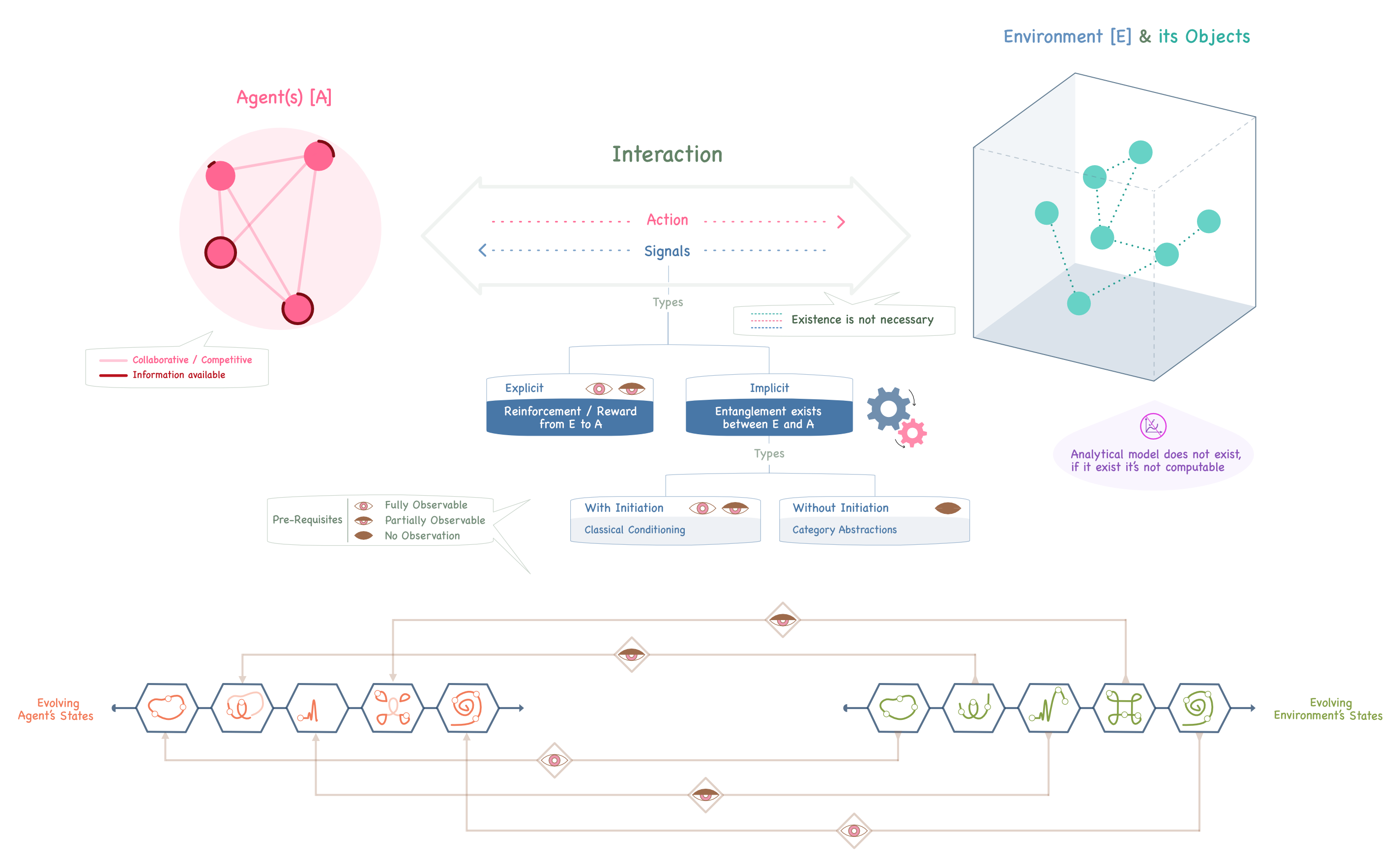
We have a set of agent(s) and an environment (consisting of multiple objects) as two disjoint entities. The aim of the agent(s) is to achieve a goal in a sequential decision-making task, under environmental constraints. The objects may collectively or non-collectively affect the environment internally, while the agent(s) collaboratively or competitively may affect the environment through external interaction, and they may share different amounts of information amongst themselves while doing so. The agent(s) would take action(s) to make their decisions, and the environment would send signals to help the agent(s). When the signals are explicit, the learning is through reinforcement, else it is through some form of entanglement between the agent(s) and the environment, which may or may not require initiation. At each instance of time, both the environment and the agent(s) have an encoding of their past history in the form of states. When the agent(s) can fully observe the environment’s states, they would normally copy them to their own state. However, when the environment’s states are only partially observable, the agent(s) may augment their state by adding a portion from their own history as well. This entire process of sequentially un-charting the environment’s functionality through state observation, actions, and signals is only required when the agent(s) do not know of a mathematical or mathematically solvable model of the environment.